A controlled study of why deep neural networks fail to train. Across 132 instrumented training runs plus a training-free propagation grid, this project measures how depth, activation, initialization, normalization, learning rate and optimizer choice decide whether useful gradients survive the trip back to the input layer.
Every experiment here is organized around one number: the per-layer propagation factor, the amount by which a single layer multiplies the backward signal.
χ=nσw2E[f′(z)2]
A network of depth L multiplies the gradient by roughly χL on its way to the input. That single exponent explains the whole corpus. A stack with χ=0.98 is fine at depth 10 and fine at depth 100. A stack with χ=0.0448 is already dead at depth 5.
Depth does not cause gradient failure — it exponentiates it. Every intervention that worked in this corpus moves χ toward 1 or breaks the product that compounds it. Every intervention that failed left χ alone.
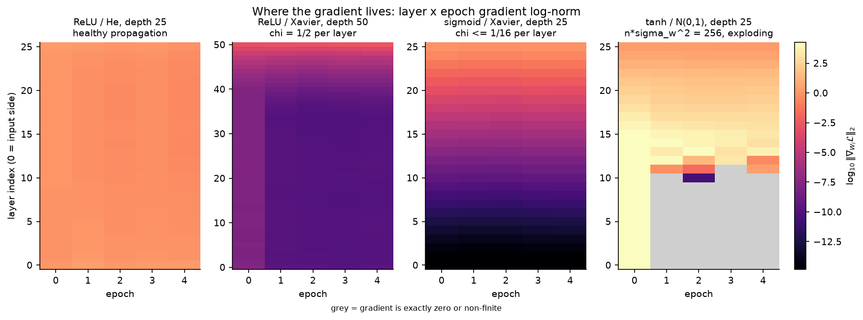
The whole study in one measurement.log10∥∇WlL∥ over (layer, epoch) for four networks. Flat colour is χ=1; the vertical ramp in panels 2 and 3 is a per-layer multiplier below 1 compounding with depth; grey marks layers whose gradient reached exactly zero in float32.
χ for every activation and initialization studied
Computed by Gaussian quadrature, not a small-signal approximation. He initialization is exactly the choice that puts ReLU at χ=1.
Bars run from χ=1. Faded bars are within 12% of 1 — the survivable regime. Note that sigmoid cannot be fixed by initialization: E[σ′(z)2]≤1/16 caps χ for any input distribution.
Experiment A · 48 runs
Where each activation breaks
Width, optimizer, learning rate and seed held fixed; only depth and the nonlinearity move. Each activation gets the initialization the literature recommends for it.
sigmoid (Xavier)tanh (Xavier)relu (He)gelu (He)
activation
survives to
fails at
propagation factor
mechanism
sigmoid
2
5
0.045
derivative ceiling, not saturation
GELU
10
25
0.979 → 0.5
He does not hold χ at 1
tanh
25
50
0.464
contractive, forward variance collapses
ReLU
25
50
1.000
χ=1, but dead units accumulate
Sigmoid fails early — and not for the textbook reason
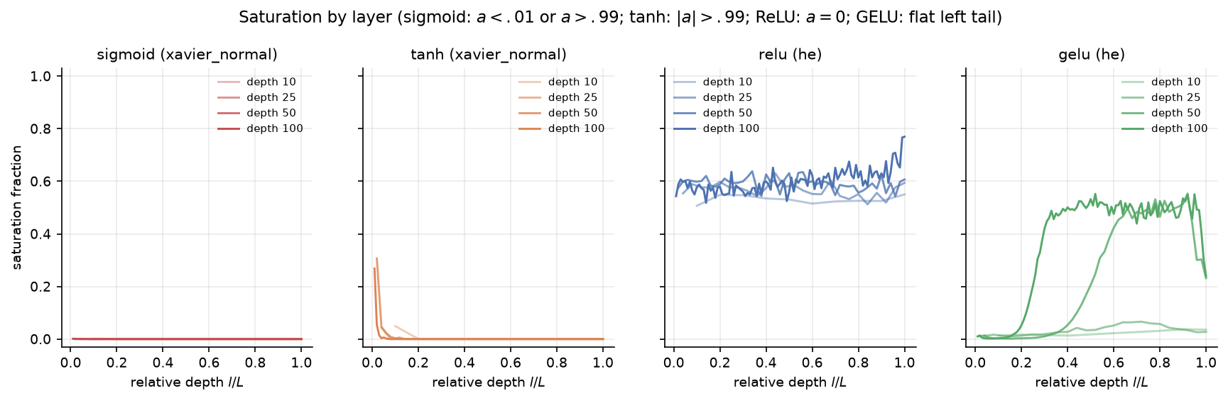
The standard explanation is saturation: units pinned near 0 or 1 where the derivative vanishes. That is not what the instrumentation shows. In the depth-25 sigmoid configuration the measured saturation fraction is 4.9e-5 — essentially no saturated units — while the gradient has already collapsed by 14.8 decades.
The cause is intrinsic and unavoidable: maxzσ′(z)=1/4, so E[σ′(z)2]≤1/16 no matter where the units sit. The contraction is multiplicative, and depth compounds it. Nothing about the input distribution can rescue it.
Measured saturation by layer. The sigmoid panel is flat at zero at every depth — the failure in the panel is real, but saturation is not its cause.
sigmoid (Xavier)tanh (Xavier)relu (He)gelu (He)
Gradient propagation ratio, ∥∇W1∥/∥∇WL∥. Points are missing where the input-side gradient underflowed to exactly zero and the ratio is undefined.
Experiment B · 20 runs
A factor of two, compounded 100 times
Xavier and He differ by exactly 2 in weight scale. For ReLU that is χ=0.500 instead of χ=1.000. At depth 10 the difference is invisible. At depth 25 it decides whether the network trains at all.
ReLU network
Xavier (χ = 0.500)
He (χ = 1.000)
gap
depth 10
0.832
0.836
+0.4 pts
depth 25
0.312
0.811
+49.9 pts
ReLU / He (χ = 1)ReLU / Xavier (χ = 0.5)
The two curves are indistinguishable until depth 10, then separate. This is what 0.5L versus 1L looks like in practice.
GELU: He does not transfer
He initialization is derived for ReLU, which is positively homogeneous. GELU is not, so E[f(z)2]=21Var(z) and the variance-preservation argument does not carry over. In this setup χ drifts from 0.979 at the first layer toward 0.5 deeper in the stack, and the forward variance collapses by layer 100. This is a statement about the configuration measured here, not about every possible GELU setup.
Experiment C · 12 runs
Normalization rescue
Four architectures that Experiments A and B showed to be broken, re-run with BatchNorm and LayerNorm inserted between every linear layer and its activation. On these four selected cases, BatchNorm rescued 3 of 4 and LayerNorm rescued 1.
broken architecture
none
BatchNorm
LayerNorm
relu d25 normal_1.0
0.105
0.485
0.588
relu d50 xavier_normal
0.100
0.118
0.182
sigmoid d25 xavier_normal
0.116
0.838
0.116
tanh d50 xavier_normal
0.215
0.789
0.176
This is a result about these four failure cases, not a general ranking. BatchNorm rescues the sigmoid stack because it re-standardizes the pre-activations every layer, breaking the χL product outright. LayerNorm normalizes across features within a sample and does not restore the same statistics here.
Experiments D & E · 52 runs
Why the learning rate cannot fix it
A vanishing gradient is often treated as something a bigger step size can compensate for. It cannot. Sweeping η across six decades moves the sigmoid stack's propagation ratio essentially not at all — the geometry of the backward pass does not depend on the step size.
Six decades of learning rate; the vanishing stack's ratio stays pinned near -15.03. Raising η only buys divergence: the ReLU network produces non-finite losses at η≥1.
Optimizers, each tuned on its own grid
Comparing optimizers at one shared learning rate only measures which optimizer likes that number, so each gets its own grid and is represented by its best result.
optimizer
healthy net (ReLU/He d10)
broken net (sigmoid/Xavier d25)
sgd
0.838
0.116 chance
sgd_momentum
0.853
0.116 chance
adam
0.860
0.105 chance
adamw
0.851
0.105 chance
An observation about Adam. Once per-element gradients fall below Adam's ϵ floor — 10−8 by default — the m^/(v^+ϵ) normalization stops being scale-invariant and the update collapses toward zero instead of rescaling. That is what was measured here with PyTorch's default ϵ; other implementations or ϵ values may behave differently.
Training-free propagation grid
Theory against measurement
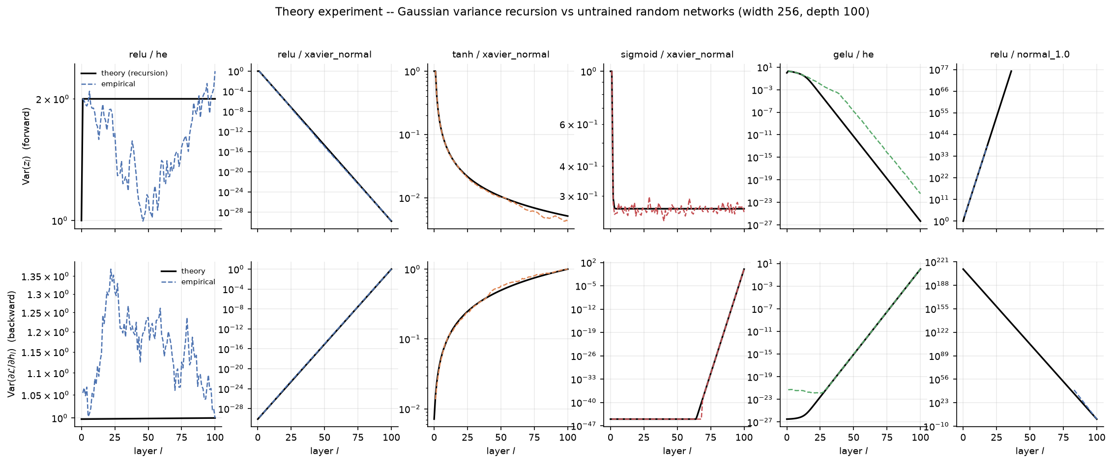
No training at all: standardized noise pushed through freshly initialized random networks up to depth 100, measured layer by layer, and compared with the Gaussian variance recursion.
ql+1=nσw2Ez∼N(0,ql)[f(z)2],q~l=q~l+1χl
Both expectations are evaluated by quadrature, so the prediction is exact under the Gaussian assumption rather than a small-signal linearization. It tracks the measurement across the full dynamic range the corpus spans — tens of decades of decay, and tens of decades of growth.
Prediction (black) against measurement (coloured). Forward variance on top, backward gradient variance below, over 100 layers, for six activation/initialization pairs.
The residual is a finite-width effect
The recursion is a large-width limit; at finite width a single network's log-variance performs a random walk around it. If the framework is right, the residual should shrink as the network widens — and it does.
tanh / Xaviergelu / Herelu / He
tanh/Xavier falls from 0.198 at n=32 to 0.006 at n=1024. ReLU/He is the marginal χ=1 case, where the log-variance walk has no restoring drift, so its residual shrinks more slowly and less smoothly.
Diagnosis engine
Automatic autopsy
Every run is diagnosed by a deterministic, rule-based engine — no model, no LLM. Thresholds are declared constants, verdicts are auditable, and the whole corpus can be re-diagnosed from disk without retraining. Across 132 runs it returned 56 healthy, 16 degraded and 60 failed.
AUTOPSY RESULT
--------------
Run: A_depth_activation__matched_sigmoid_d25__5e0b80effe
Status: Failed

Architecture:
25 x 256 sigmoid, init=xavier_normal, norm=none, sgd lr=0.05

Gradient attenuation:
output -> input gradient ratio = 1.58e-15 (log10 = -14.80)
||grad W_first|| = 1.43e-15, ||grad W_last|| = 7.92e-01

Activation propagation:
Var(h_L)/Var(h_1) = 2.89e-01 (log10 = -0.54)

Parameter updates:
first 18 layers update/weight < 1e-07
Parameter updates have stalled in 18/26 linear layers (update/weight < 1e-07); the first 18 layers are frozen.

Learning outcome:
validation accuracy 0.0930 (chance 0.1000), final train loss 2.3173

Findings:
  [critical] vanishing_gradient: Gradient attenuates toward the input: output -> input gradient ratio = 1.58e-15.
  [critical] stalled_updates: Parameter updates have stalled in 18/26 linear layers (update/weight < 1e-07); the first 18 layers are frozen.
Three rules that came from the data
These exist because real experiment output broke simpler assumptions — the part of the work that only shows up once you run the corpus.
Gradient extinction. When the input-side gradient underflows to exactly zero in float32 while the output side is still alive, log10 of the ratio is undefined and a plain ratio test silently misses the most severe case there is. Extinction is now detected and reported separately from ordinary vanishing. 7 runs in the corpus are in this state.
Trigger disambiguation. A finding raised by an absolute gradient norm must not claim that a ratio exploded. One Adam run reported “amplifies toward the input” alongside a ratio of 0.25; the rule now names which test actually fired.
Partial learning. A network that crawls above chance is not healthy. A run whose validation loss falls to only a modest fraction of its starting value is reported as partial_learning rather than waved through — 10 runs land here.
Boundaries
What this does not show
Architecture. MLPs only, on flattened images, with no skip connections — the standard fix for exactly this problem, deliberately out of scope. These findings do not automatically transfer to residual networks, convolutional networks or Transformers.
Data. Fashion-MNIST and a synthetic Gaussian mixture, not large modern benchmarks.
The χ framework rests on mean-field variance-propagation assumptions — independent weights, Gaussian pre-activations by CLT over the width. It describes this regime well; it is not offered as an architecture-independent law.
Finite width. The recursion is a large-width limit; deviations at width 256 are quantified in the width sweep rather than hidden.
Normalization conclusions come from four selected failure cases, not a general comparison of BatchNorm and LayerNorm.
Optimizer results depend on implementation and hyperparameters — PyTorch defaults, per-optimizer learning-rate grids, a five-epoch budget.
Numerics. float32 throughout, with subnormals deliberately preserved rather than flushed, so recorded gradients are the true float32 values. The associated runtime behaviour is CPU-dependent.
Budget. One seed per trained configuration. The conclusions concern where propagation breaks, not final attainable accuracy.
Reproduce
Verification in three minutes, or the full corpus in 4.3 hours
The fast path needs no training corpus: it runs the test suite, exercises the entire pipeline on four tiny networks, and re-checks every number quoted in the report against the generated tables.
The full corpus, if you want it — about 4.3 hours of wall clock on the documented CPU, of which 4.2 h is recorded training time and the rest is the training-free theory grid and initialization audit:
python -m gradient_autopsy.experiments.run_all   # 132 runs
python -m gradient_autopsy.figures               # rebuild all figures
streamlit run app/streamlit_app.py               # interactive explorer
A systems note. Runtime is dominated by the dying networks, not the deep ones. Once gradients enter the float32 subnormal range, CPU arithmetic slows by one to two orders of magnitude — a depth-25 sigmoid run takes 329 s while a depth-50 one takes 13 s, because the deeper network underflows all the way to exactly zero, and zero is fast. Runtime is not monotonic in depth. This is a property of the tested CPU; other hardware handles subnormals differently.